Computation With The World’s Smallest Programming Language

Update: The latest version of the lambda calculator has line editing and a command history. It’s more convenient than the version linked in the blog and is tagged 0.1.0.

Note to the reader: much of this post is based on an article I found on the web called Lambda Calculus (part I). That article covers the material here in more depth and more coherently.

In The World’s Smallest Programming Language I started describing the Lambda Calculus. At this point, we need to describe how to do things with it. How do we compute with The Lambda Calculus?

Rewriting Expressions

We do computation in The Lambda Calculus by rewriting expressions according to various rules, well, actually two rules. The first one is as follows:

1. Identify an application in which the first term is an abstraction.
2. Replace the occurrences of the abstraction’s parameter in its body with the second term of the application.
3. Replace the application with the modified body of the abstraction.

Note: an application that has an abstraction as its first term is called a reducible expression, or redex for short. The name is slightly misleading because you don’t necessarily end up with an expression that is reduced in size or complexity, but we are stuck with it.

Here is an example:

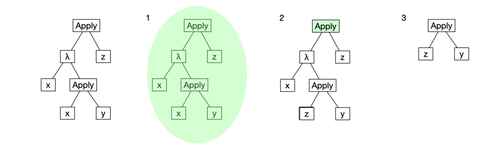
: (λx.x y) z
> 
: z y

Here, we started with the expression (λx.x y) z which is an application of an abstraction λx.x y to a variable z. The parameter of the abstraction is x so we can rewrite it by replacing the occurrences of x in the abstraction with z. Sometimes it’s easier to understand if you draw out the structure of the expression as a tree, like this:

Multiple Redexes and order of rewriting

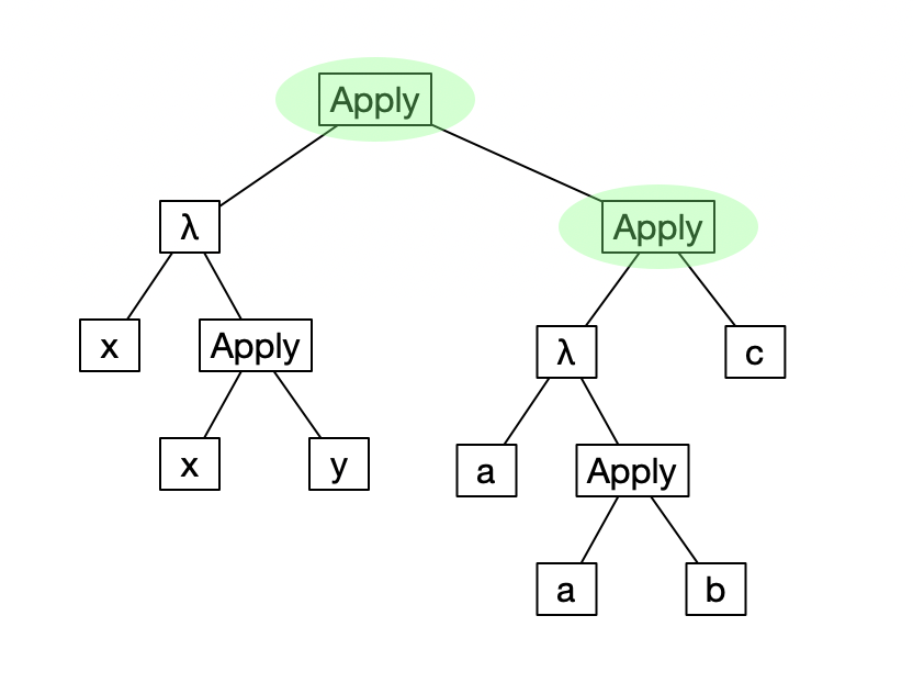
Frequently you have more than one redex, for example:

 (λx.x y) ((λa.a b) c)

This has the following structure with two redexes (highlighted in green).

If we run it though my lambda calculator, we get

: (λx.x y) ((λa.a b) c)
> 
: (λa.a b) c y
> 
: c b y

It’s chosen to do the left rewrite first and then do the right one. On a diagram, it looks like this:

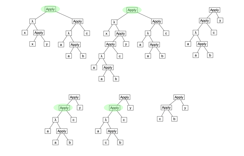
If the lambda calculator had chosen to do the right one first, it would look like this:

: (λx.x y) ((λa.a b) c)
> 
: (λx.x y) (c b)
> 
: c b y

In this case, it gets the same answer, but the order you choose to do things in can have profound consequences. Consider  (λx.y) ((λz.z z) (λz.z z)). Here we have a choice of two redexes to rewrite. We could choose to rewrite the outermost application, in which case it reduces immediately to y and you can’t go any further. This is because the parameter of λx.y doesn’t appear in its body. However, if we choose to reduce the second term of the outermost application (λz.z z) (λz.z z) which is also a redex, we get (λz.z z) (λz.z z) which is itself. If we always choose the right hand side to rewrite, we’ll never get anywhere.

For this reason, the lambda calculator uses a strategy of “left most outermost” or “normal order” to pick a redex to rewrite. Essentially, it starts at the top of the tree representing the expression. If it’s a variable there aren’t aren’t any redexes. If it’s an abstraction it descends into the body of the abstraction and repeats. If it’s an application and the application is a redex, this is the expression chosen, otherwise it repeats the process with the first (or left) term and only searches the second (or right) term if it fails to find a redex on the left side. This guarantees that, if an expression can be reduced by successive rewrites to a point where there are no redexes left, it will be.

This state where there are no redexes left, is called normal form hence the alternate name of “leftmost outermost”. Note that using leftmost outermost reduction does not guarantee you will ever reach a normal form. The expression above where you get the same expression back cannot be reduced to the point where there are no redexes left. Even worse: (λz.z z (z z)) (λz.z z (z z)) just gets bigger and bigger.

Using normal order reduction provides you with the best chance of getting an expression in normal order form, but the advantage comes at a cost. Consider  (λx.x x) ((λy.y) z). If we reduce it, we get

(λx.x x) ((λy.y) z)
> 
: (λy.y) z ((λy.y) z)
> 
: z ((λy.y) z)
> 
: z z

It takes three reductions to get to a normal form. If we chose a strategy where we evaluate the second term (or argument) of the outermost application, it would go like this:

(λx.x x) ((λy.y) z)
> 
: (λx.x x) z
> 
: z z

It would only take two reductions because we evaluate the argument before we duplicate it. This is called leftmost innermost reduction or applicative order reduction. Essentially, it’s the difference between evaluating the function first or evaluating the the argument first. In normal computer programming, the analogue would be call by name versus call by value, or, thinking about Swift in particular, the difference between normal function calls or function calls passing a closure.

Hazards of Rewriting

I want to talk about two problems that come about due to the naive application of the rewriting rules above. Before we start, I should point out that the lambda calculator has already been fixed to avoid these problems and if you try running the examples, you’ll see different and correct output compared to what is here.

Problem #1: Consider (λx.(x p ((λx.x p 1) 3))) 2. If we rewrite it using the rules I have described so far, using normal order reduction, it would go something like this:

: (λx.x p ((λx.x p 1) 3)) 2           [1]
> 
: 2 p ((λx.2 p 1) 3)                  [2]
> 
: 2 p (2 p 1)                         [3]

[1] is the original expression. [2] is the expression after rewriting the outermost redex, replacing instances of x with the argument 2. [3] is the result of rewriting the other redex replacing the instances of x with the argument 3 (there aren’t any left, as it happens). You may ask what is the problem with that? Well the answer is that p in this case was chosen to stand for “plus” and the original expression is meant to stand for (λx.x + ((λx.x + 1) 3)) 2 and the answer ought to be 6. Indeed, if we used applicative ordering, it would look like this:

: (λx.x p ((λx.x p 1) 3)) 2           [1]
> 
: (λx.x p (3 p 1)) 2                  [2]
> 
: 2 p (3 p 1)                         [3]

You’ve probably spotted that the problem here is one of scoping: the x in the inner abstraction is not the same x as the one in the outer abstraction and we shouldn’t have replaced it when we rewrote the outer abstraction.

Problem #2: The second problem is exemplified by the following:

: (λx.λy.x) y z                       [1]
> 
: (λy.y) z                            [2]
> 
: z                                   [3]

[1] is the original expression. [2] is the result of rewriting the outermost redex and [3] is the result of rewriting the new redex created by [2]. What’s wrong with that? Well, the correct answer should have been y. The reason for this is due to the concept of α-equivalence (“alpha equivalence”). The name of an abstraction’s parameter shouldn’t really matter, for example: λx.a b c x d e and λp.a b c p d e, when used as a function in a redex, give the same result for all arguments. Intuitively we think of these as the same abstraction. The name for this intuitive relation is α-equivalence. α-equivalence says, in simple terms, that the name of the parameter of an abstraction doesn’t really matter, as long as you don’t rename it to clash with another variable in the abstraction and you rename it consistently throughout the abstraction. So, if we rename the parameter of the inner abstraction to give us e.g. (λx.λp.x) y z, we expect the same result as before, but it would go:

: (λx.λp.x) y z                       [1]
> 
: (λp.y) z                            [2]
> 
: y                                   [3]

The problem here is that the y we substitute in during step [2] of the original expression is a different y to the y that is the parameter of the abstraction.

Bound and Free Variables

The solution to these problems comes in the form of α-reduction and β-reduction. To understand α-reduction and β-reduction, we need to understand what a bound variable is.

• A bound variable is a variable that appears as a parameter in an enclosing abstraction
• A free variable is a variable that is not bound

In (λx.λy.x y) y z, x is bound. y appears twice. In the first case , it is bound as part of the abstraction λx.λy.x y but in the second case it is free because it is outside of that abstraction.

The first problem above is easily solved with the following refinement to the rewriting rule:

1. Identify an application in which the first term is an abstraction.
2. Replace the occurrences of the abstraction’s parameter that appear free in its body with the second term of the application.
3. Replace the application with the modified body of the abstraction.

That is: in (λx.M) N replace occurrences of x that are free in M with N. In our example

(λx.x p ((λx.x p 1) 3)) 2

M is x p ((λx.x p 1) 3) and N is 2. Only the first occurrence of x in M is free, so we only replace that occurrence with 2. We leave the other one alone.

The second problem is solved by finding all the abstractions in the body of the function that would cause any of the free variables in N to become bound and find an α-equivalent form that does not do this. Insert this step between steps 1 and 2. Slightly more formally, in a redex λx.Μ Ν if M contains an abstraction λy.P and y is free in N, pick a name y' such that y' does not appear free in P or N and replace the parameter of λy.P and all free occurrences of y in P with it. This is called α-reduction. The lambda calculator does α-reduction automatically, when necessary.

: (λx.λy.x) y z    [1]
> 
: (λy'.y) z        [2]
> 
: y                [3]

Our new rewriting rule is

1. Identify a redex according to the ordering rule you chose. This redex is of the form (λx.M) N
2. α-reduce the abstraction λx.M such that it does not have the same name as any variable that appears free in N. Call it x'.
3. Replace the occurrences of x' that appear free in M with N.
4. Replace the application with the modified body of the abstraction.

This is called β-reduction, and it’s the only rule you need (or that exists) to do computation in the Lambda Calculus.

This concludes today’s post. In the net post, I will explain how you can model more traditional computing idioms.